The
graphical representation of a normal distribution is a bell-shaped curve that
is symmetrical about the mean. Therefore, half of the values of the random variable X are equal to or
greater than the mean and half are equal to or less than the mean. The curve
encompasses 100% of the population with all possible values that the random variable can assume liyng under the
curve. A normal distribution is defined by two parameters: the mean, denoted by
µ and the standard deviation, denoted by σ.
Graphical representation of the normal distribution
EXERCISES
On
a certain road, the speed limit is 40 km/h with a tolerance of 7 km/h. The
speed at which the driver travels on this road varies, with an average speed μ=40km/h
and a standard deviation σ = 4 km/h. What is the
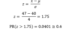
probability that the driver will exceed 47 km/h and get a ticket? To determine this, we must
standardize the variable (µ = 0, σ =1. Then we can consult a
standardized normal distribution table, typically located at the end of
statistical textbooks. Calculate:
Tip: You can utilize software to determine probabilities..
2. In regular operation conditions, radar readings is a random variable normally distributed with mean μ = 25 mph and standard deviation σ = 3 mph. To test the calibration of the radar, a test car traveling at 25 mph is used. Assuming the radar is correctly calibrated, i.e., with μ = 25 mph and σ = 3 mph, what is the probability that the radar detects the test car’s speed to be: a) 28 mph or higher? b) 27½ mph or higher? c) At what speed should the radar record for the probability of a value exceeding this speed to be 5%?
a) Probability of detecting 28 mph or more.
c) To have a 5% probability of the radar measuring a higher speed.
Remember that
More control means fewer mistakes. You need to keep this in mind when
you want more quality. Compare the probabilities obtained in examples 2b, 3 and
4.
3. A calibration test will be carried out on 4 radars that operate together. A test car with a speed set at 25 mph will be used. Under optimal conditions, the speed of each radar is a random variable following a normal distribution with mean µ=25 mph and standard deviation σ=3mph. If the radars are calibrated, what is the probability that the collected measurements will give an average speed of 27½ mph or higher?
4. The idea of using 4 radars is good; however,
having 9 is advantageous. Increased control (in this case, through a larger quantity of radars) decreases the risk of error. There are 9
calibrated radars in operation
simultaneously. After calibration, the speed of each radar unit is a normally distributed random variable
with mean µ = 25 mph and standard deviation σ = 3 mph. Using a test
car traveling at a constant speed of 25
mph, what is the probability that the collected measurements will yield
an average speed 27½ mph or higher?
OPERATIONS OF RANDOM VARIABLES
If X and Y are independent random variables with means µ1 and µ2 and variances σ12 and σ22 respectively, then:
Z = X + Y is a random variable with mean µ1 + µ2 and variance σ12 + σ22.
W = X – Y is a random variable with mean µ1 – µ2 and variance σ12 + σ22.
Var (a Z) = a2 Var (Z)
σ (a Z) = a σ (Z).
EXERCISE
5. If we consider the subway arrival time as a random variable with mean µ1 = 8h10m and standard deviation σ1 = 40s, and your arrival at the station as a random variable with mean µ2 = 8h08m and standard deviation σ2 =30s, how likely is it that you will miss the train? Let S represent the subway arrival time and Y represent your arrival time at the station. Therefore, W = S – Y, your waiting time, is a random variable with a normal distribution, having an average of 8:10 – 8:08 = 2 m = 120 s, variance of 402 + 302 =1600 + 900 = 2500 s, and a standard deviation of 50. Missing the train would occur if W ≤ 0. To calculate the probability of W ≤ 0:
Decision rule
Set critical values to reject specific results. This is crucial for quality control.
EXERCISE
6. In
the canning
industry, the pH (the acidity) of the product in each can is a random variable that is normally distributed with mean 7 and standard deviation of 0.5. If the pH of the product falls
below 6.0 or exceeds
8.0, the can is rejected. What is the
probability of this happening?


